We present a compact, physically-based model that faithfully emulates the colour response of positive photographic film from a digital RAW image. Unlike hand-crafted look-up tables (LUT) or data-hungry neural networks, our approach analytically mirrors the film “capture-develop–scan” chain, all with around 30 trainable parameters. Least-squares optimisation on 3168 colour patch pairs captured on one roll of Fujifilm VELVIA 100 achieves colour chart root-mean-squared-error (RMSE) 1.3 % with no interpolation artefacts. Additionally, qualitative comparisons show the proposed model more closely matches real film than Fujifilm’s proprietary VELVIA “film simulation”. The continuous model can also be discretised into LUTs of any resolution, offering production-ready film emulation and a path for archival of discontinued stocks.

SIGGRAPH Posters 2025 Abstract

SIGGRAPH Posters 2025 Poster (Also Below)

Source Code (Coming Soon)

Acknowledgements

I’m extremely grateful to Professor Michael Brown and Dr. Hakki Karaimer for their guidance and feedback, as well as Professor Kyros Kutulakos for giving me a chance to begin this project.

Introduction

Motivation

Photographic film emulation is widespread among both camera manufacturers and photographers. Even after digital sensors overtook film, decades of research and development devoted to “pleasing” film colour were transplanted into digital picture styles. Today, photographers who never touched film still pursue its look: hundreds of Adobe Lightroom “Film Presets” exist, and Fujifilm’s in‑camera “Film Simulations” remain best‑sellers (Artaius, 2024). Yet most emulation workflows are limited to (1) manual tweaks in an editor, (2) opaque LUT mappings, or (3) proprietary pipelines hidden from the public. To overcome such limitations, we propose a model that is accurate, concise and physically grounded.

Goals

Our model targets the core colour and tone‑forming stages of a colour‑positive film workflow so that a digital RAW file can be processed to match a chosen film stock. Design criteria are:

1. Accuracy with simplicity: a small parameter set that can be fitted robustly, all while sufficiently encoding the target film’s chromatic and tonal properties.
2. Minimal data capture: one 36‑exposure roll plus a colour chart with patches should be all that is required, with no pixel-perfect alignment.
3. Physical grounding: parameters map to real film behaviour, ideally confirmed with known properties of the film.

Non‑colour artefacts such as grain, halation and flare are outside our scope, and we focus on colour‑positive film only.

Related Work

Radiometric Calibration for Digital Cameras

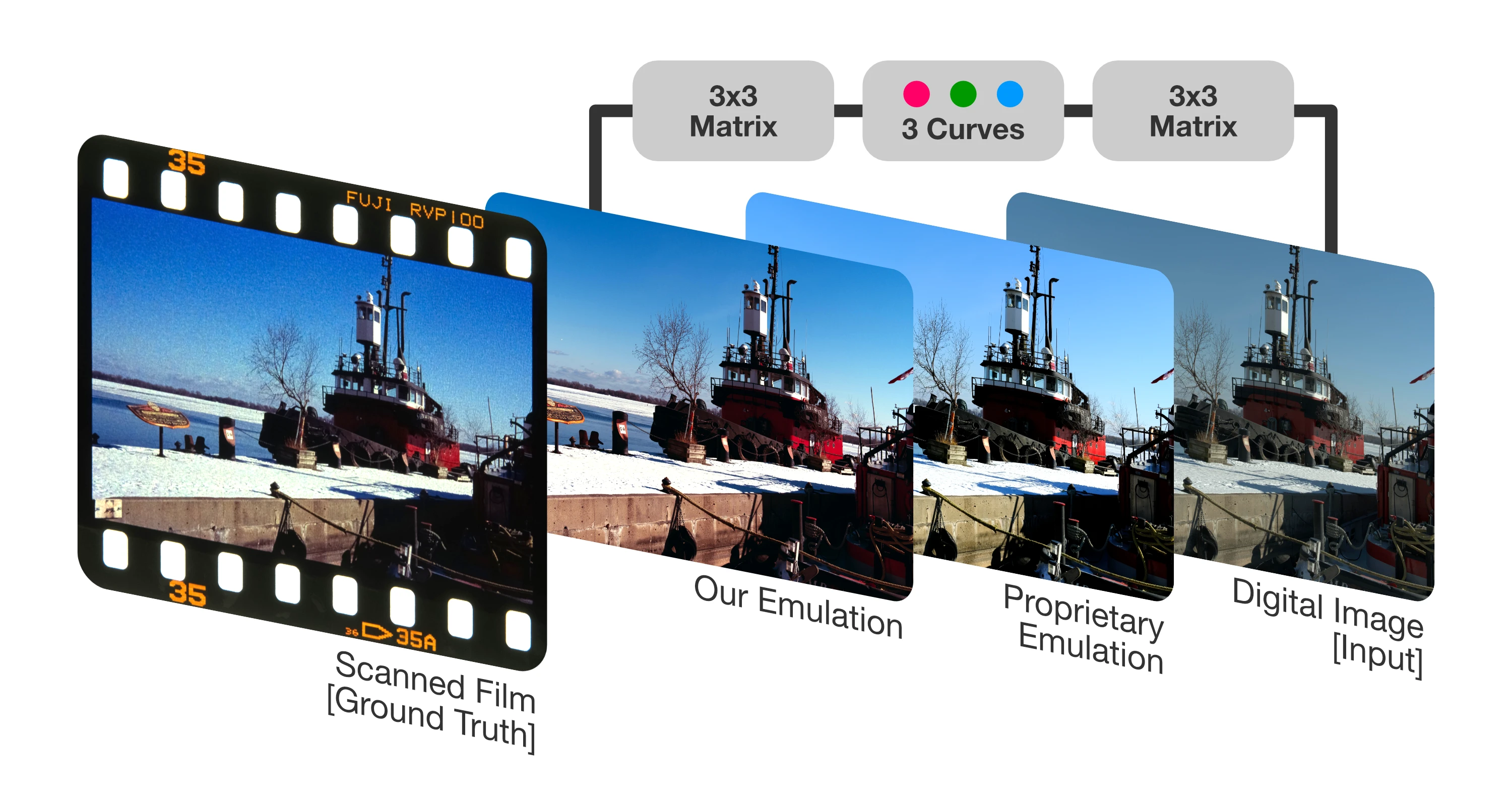
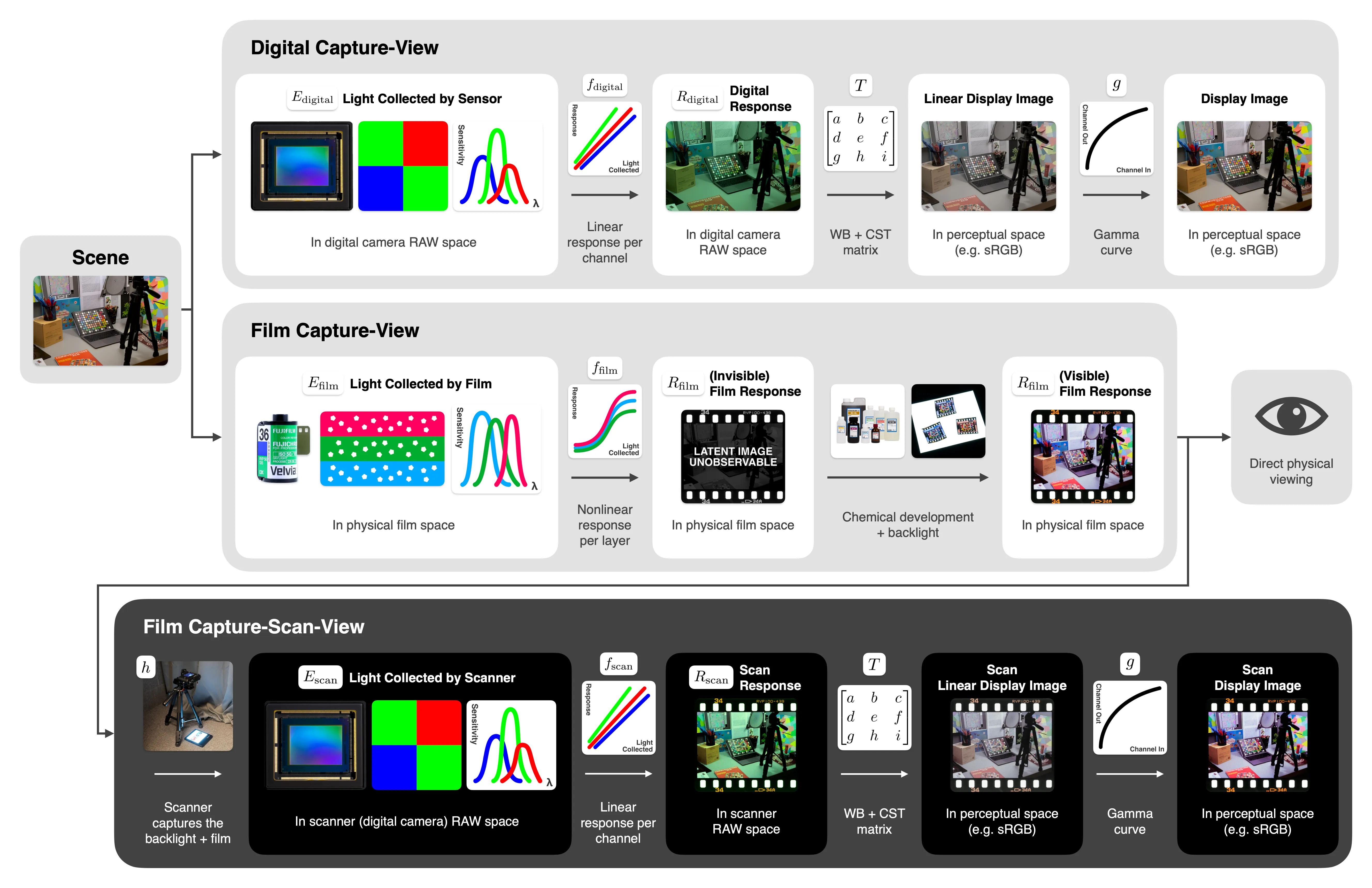
“Radiometric calibration” is the process of estimating a digital camera’s in‑camera pipeline: tone curves, white balance (WB), colour‑space transforms (CST) and gamut mapping, so that RAW images can be reconstructed from, or mapped to, processed images. Classic methods (Lin et al., 2011; Kim et al., 2012) model the chain with two $3 \times 3$ matrices for WB and CST, a nonlinear gamut‑mapping term implemented via radial‑basis functions (RBF) and three per‑channel tone curves. These models accurately reproduced proprietary styles and recovered RAW data for several commercial digital cameras. Similarly, our goal is to transform a digital RAW into the RAW that a scan of a specific colour‑positive film would yield. But simply transplanting a digital camera model to film is inadequate. Film introduces an analogue capture stage, chemical development and a separate scanning step; radiometric calibration pipelines omit this extra capture, as detailed in Section Consequence of Scanning.

Film‑Process Modelling

Early work (Bakke et al., 2009) paired colour chart images shot with both digital and film cameras, then fitted a polynomial from the digital RGBs to the scanned‑film RGBs. Recent efforts employ neural networks: FilmNet (Li et al., 2023) trains a multi‑scale U‑Net on 5000 synthetically generated digital-“film” pairs, while (Mackeenzie et al., 2024) uses an end‑to‑end convolutional neural network (CNN) on generic image pairs. Photographic community projects include LUT construction from known colour patches (David, 2013) and small multilayer perceptrons (MLPs) trained on synthetic Fujifilm “Film Simulation” RAW-JPEG pairs (Anonymous, 2024). Across these approaches, a black‑box function is fitted directly between digital input and scanned‑film or synthetically emulated film output. Such models are neither physically grounded nor interpretable, and it is difficult to confirm whether they model the target film accurately. Moreover, most rely on synthetic film images (i.e. the training images are also emulations); only (Bakke et al, 2009; Mackeenzie et al., 2024) use real scans, and even they treat the scanning pipeline as part of the black box.

Photographic‑Style Estimation

Style‑transfer research offers more general solutions. A differentiable network in (Tseng et al., 2022) learns slider parameters compatible with Adobe Camera RAW, while (Hu et al., 2018) can infer a style from exemplar images alone, eliminating the need for paired data sets. These frameworks are powerful but overly general for film: by constraining the domain to colour-positive film colour, we can craft a much simpler model and a lightweight data collection routine.

Preliminaries

Film Spectral Sensitivities

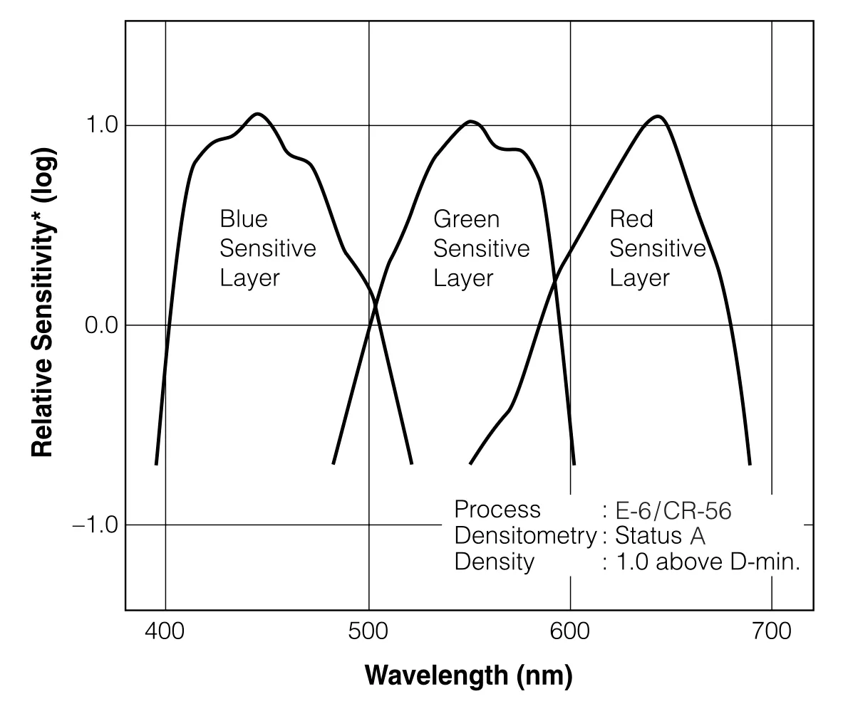
Colour film comprises three dye‑coupled silver‑halide layers, each with its own spectral sensitivity to incoming light (exposure). That is, each layer will “collect” light from a specific range of wavelengths. Such spectral sensitivities contributes to a film’s “look”, analogous to a digital sensor’s colour‑filter array (CFA) and its sensitivities.

Film Characteristic (Response) Curves

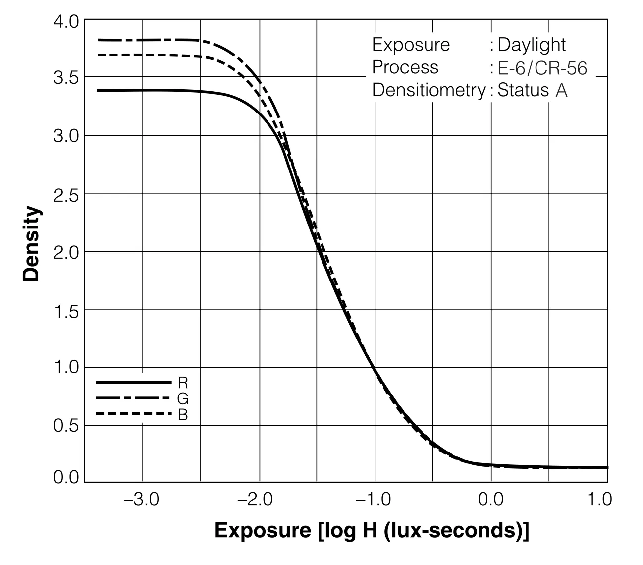
Once a film layer is sensitised by incoming light (exposure), they result in a certain response, also known as optical density. In layman’s terms, the amount of exposure determines whether a layer becomes dark (opaque) or transparent. For film, exposure response follows an S‑shaped curve, also called the characteristic curve. Whether a curve is increasing or decreasing is determined by the film’s type:

• Colour‑negative (top) film records an inverted image with an orange base layer, which must be then printed on photographic paper or scanned and inverted digitally.
• Colour‑positive (bottom) film records a transparent image that can be viewed over a backlight.

Unlike film, modern digital sensors have a mostly linear response to exposure. For example, if the exposure was 1 (arbitrary unit) and the resulting value recorded was 100, an exposure of 2 would result in a value of 200. This is not true for film.

Consequence of Scanning

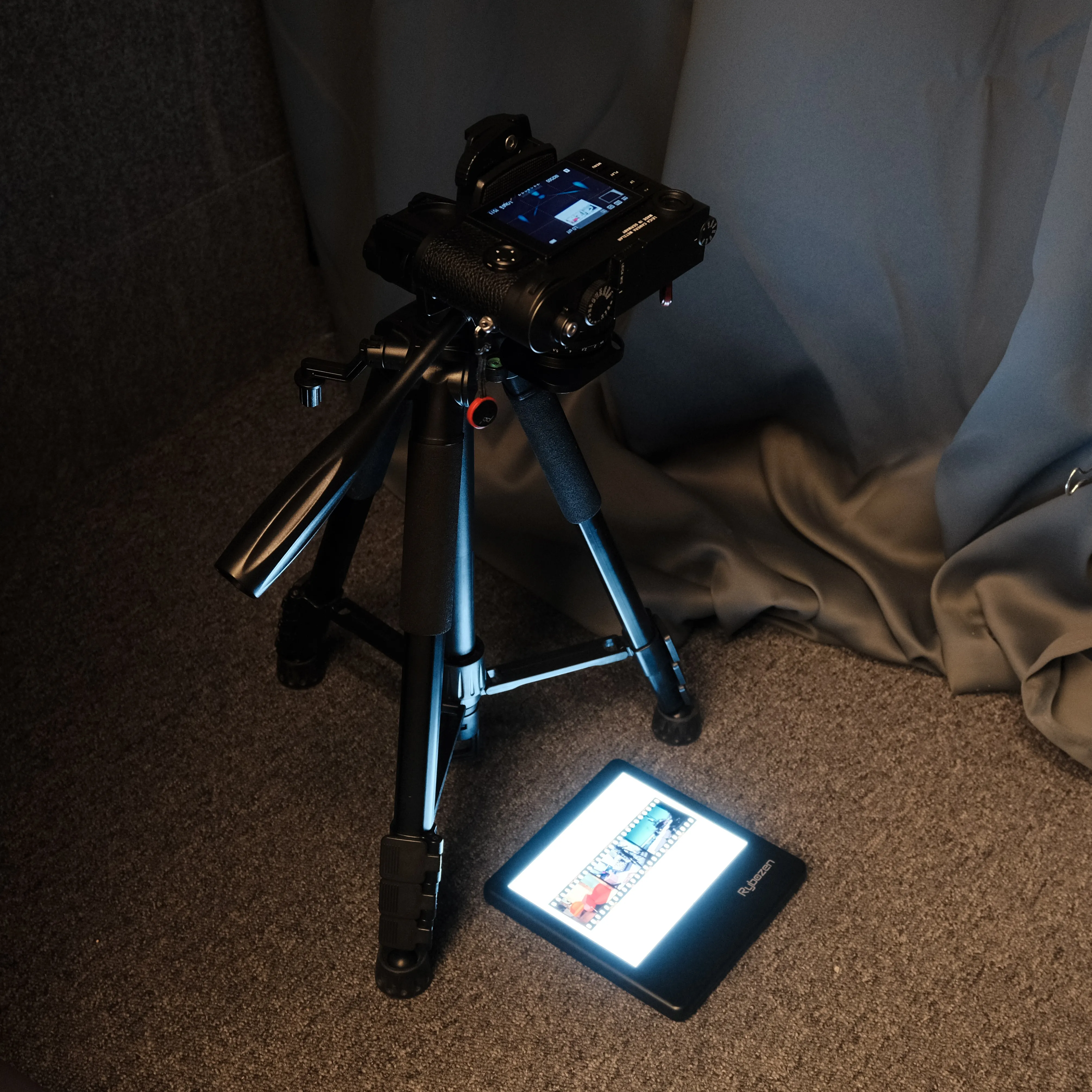
Historically, film was either printed on paper (colour-negative) or viewed over a backlight (colour-positive). Nowadays, many capture the developed frame with a digital camera or scanner, introducing a second digital capture stage after the original capture. In our emulation we will specifically deal with colour-positive film on top of a backlight, which is then captured with a digital camera.

Overview of Digital, Film and Scanned Film Pipelines

For the remainder of this work, we adopt the following symbols (device $x \in {\mathrm{digital}, \mathrm{film}, \mathrm{scan}}$):

• $E_x$: channel/layer‑wise collected light; i.e. exposure.
• $f_x$: per‑channel response (linear for $digital, scan$; S-shape for $film$).
• $R_x = f_x(E_x)$: Response to the collected light (RAW image for $digital, scan$, physical optical density for $film$).

These definitions lay the groundwork for the model in the next section.

Method

Formal Problem Statement

Our proposed workflow is as follows:

1. We capture a scene using a digital camera, which produces a RAW image.
2. We process the RAW image using our model, which gives as a RAW image that is an emulation of what we would produce if we captured the scene with a film camera, developed the film, and digitally scanned the film.
3. We apply basic WB + CST matrices and a gamma curve to make the image ready-to-view on a digital screen.

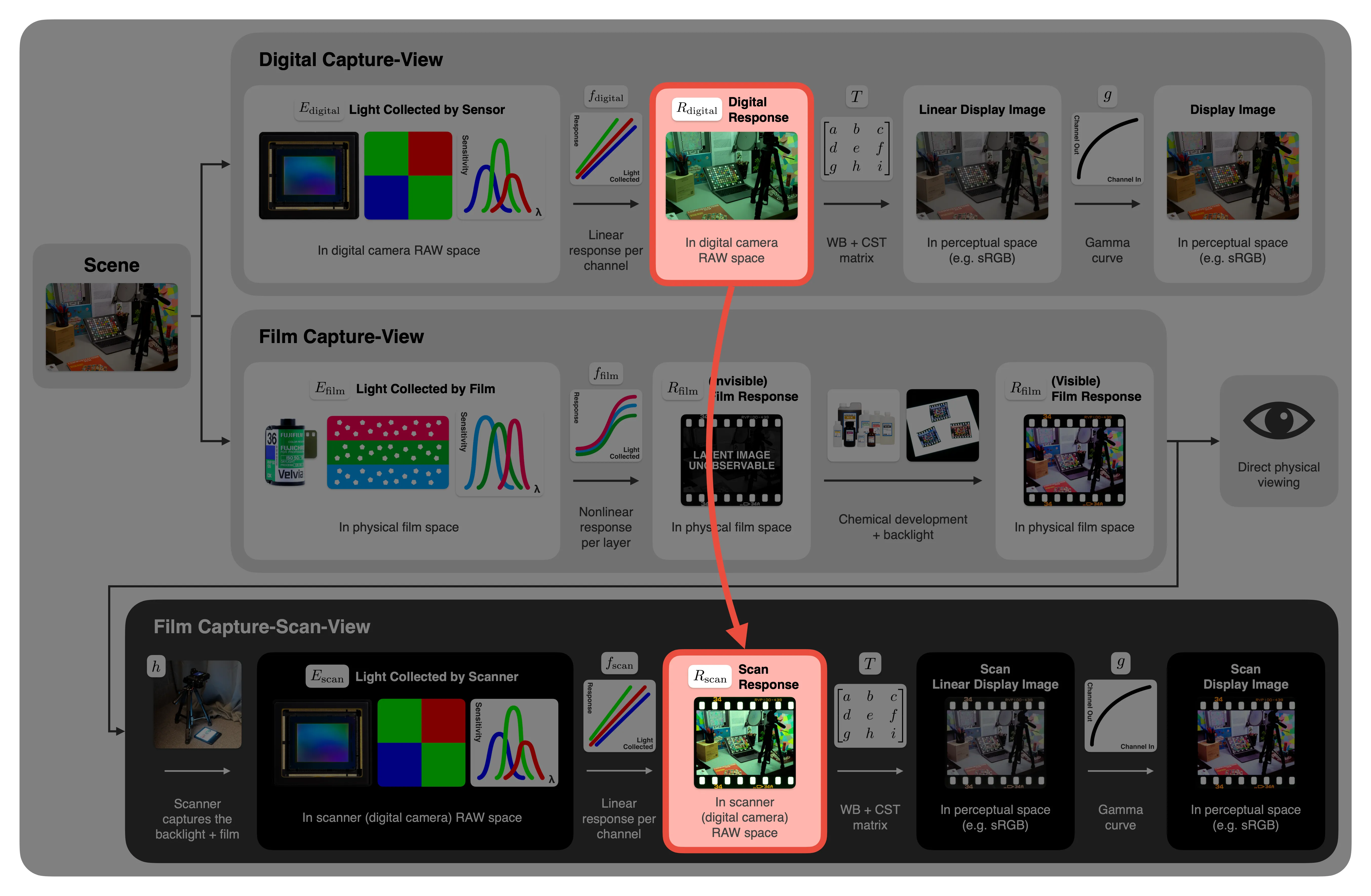
Therefore, our objective is to transform a digital‑camera RAW $R_\mathrm{digital}$ into an emulated scanned film RAW $R_\mathrm{scan}’$ so that $R_\mathrm{scan}’ \approx R_\mathrm{scan}$. This is a RAW‑to‑RAW mapping, avoiding gamut‑clipping complications and keeps the model early in the pipeline. Section Working in a Device‑Independent Space discusses alternative wide‑gamut spaces.

In the context of the overview diagram from before, we aim to map between the two images highlighted in red:

Scanned Film Emulation Model

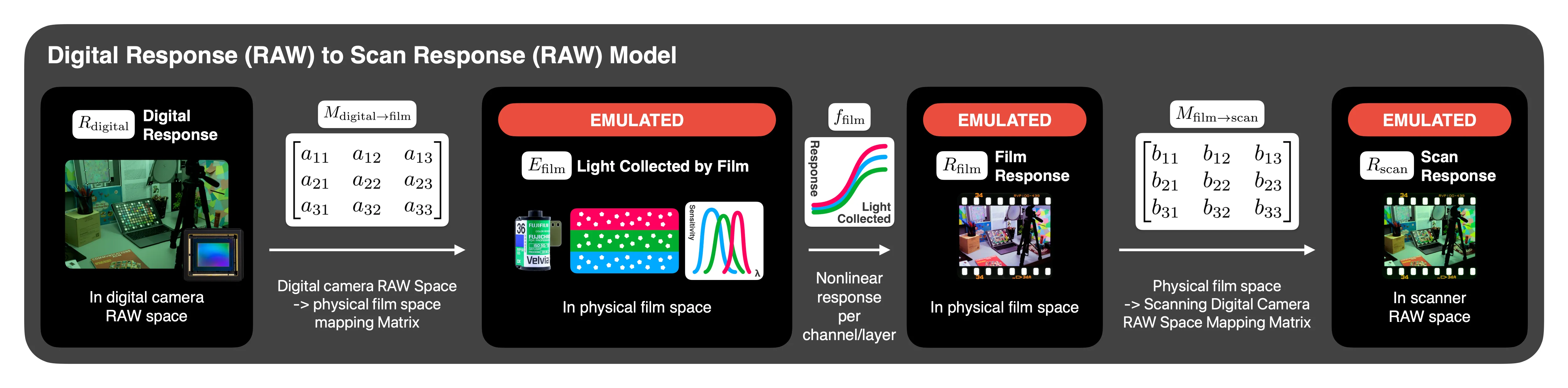
The model mirrors the physical “capture-develop-scan” process in three steps. Given a digital RAW image input $R_\mathrm{digital}$:

1. Undo the digital response: Modern digital sensors respond linearly: $E_\mathrm{digital} \propto R_\mathrm{digital}$. From there, mapping that exposure into the film’s spectral domain is equivalent to mapping between two “sensors” of different spectral sensitivities. Thanks to Grassman’s Law, this is a linear operation. Combined, we represent this step of the process with a $3 \times 3$ matrix $M_{\mathrm{digital} \rightarrow \mathrm{film}}$:

\[E_\mathrm{film}’ = M_{\mathrm{digital} \rightarrow \mathrm{film}}\,R_\mathrm{digital}.\]

1. Emulate the film response:  Each film layer exhibits an S‑shaped characteristic curve $f_{\mathrm{film}, \mathrm{channel}}’$. Following Kodak guidelines (Eastman Kodak Company, 1999), we use a per‑channel sigmoid in log exposure:

   \[R_{\mathrm{film},\mathrm{channel}}’ = f_{\mathrm{film}, \mathrm{channel}}’(E_{\mathrm{film},\mathrm{channel}}') = \frac{A}{1 + e^{-k(E_{\mathrm{film},\mathrm{channel}}' - x_0)}} + y_0,\]

   with four parameters $(A,k,x_0,y_0)$ per $\mathrm{channel}\in{r,g,b}$.

2. Emulate the scan: At this stage, we are still representing values in terms of the film’s emulated per-layer response (optical density) and we need to map them into the emulated scanner’s RAW values. Because backlights are simple, fixed-brightness illuminants, we may assume that $E_\mathrm{scan}’$, the light collected by the scanner’s sensor, is simply linear to the film optical densities $R_\mathrm{film}’$. As established, $R_\mathrm{scan}’$ is simply linear in $E_\mathrm{scan}’$ as well. Combined, we have another $3 \times 3$ matrix $M_{\mathrm{film} \rightarrow\mathrm{digital}}$ such that:

\[R_\mathrm{scan}’ = M_{\mathrm{film} \rightarrow\mathrm{scan}}\,R_{\mathrm{film},\mathrm{channel}}’.\]

The complete transformation is therefore:

\[R_\mathrm{scan}’ = M_{\mathrm{film} \rightarrow\mathrm{scan}}\,f_\mathrm{film}'\!\bigl(M_{\mathrm{digital} \rightarrow \mathrm{film}}\,R_\mathrm{digital}\bigr),\]

with 30 parameters (9 + 12 + 9) and 36 if including bias terms for the two matrices.

Key Difference from Digital Radiometric Calibration

Digital‑camera pipelines use WB + CST -> nonlinear tone curves -> (optionally) nonlinear gamut mapping. Our film model replaces the arbitrary nonlinear tone curves with physically motivated sigmoids and adds the second matrix $M_{\mathrm{film} \rightarrow\mathrm{scan}}$ after the characteristic curves stage to account for the extra scanning step absent in digital‑only workflows.

$M_{\mathrm{digital} \rightarrow \mathrm{film}}^{-1}$ in place of $M_{\mathrm{film} \rightarrow\mathrm{scan}}$

When the same digital camera both photographs the scene and scans the developed film, the two spectral‑sensitivity sets coincide. In that case, $M_2$ can be replaced by $M_1^{-1}$, dropping 9 (12 if including bias) parameters with negligible loss of accuracy (see Section Experimental Results).

Parameter optimisation

We jointly fit all parameters with nonlinear least‑squares on a dataset of 3168 colour‑patch correspondences captured on a single 36‑exposure roll of Fujifilm VELVIA 100. From there, SciPy’s least-squares optimiser converges reliably from zero‑initialised parameters.

Data Collection

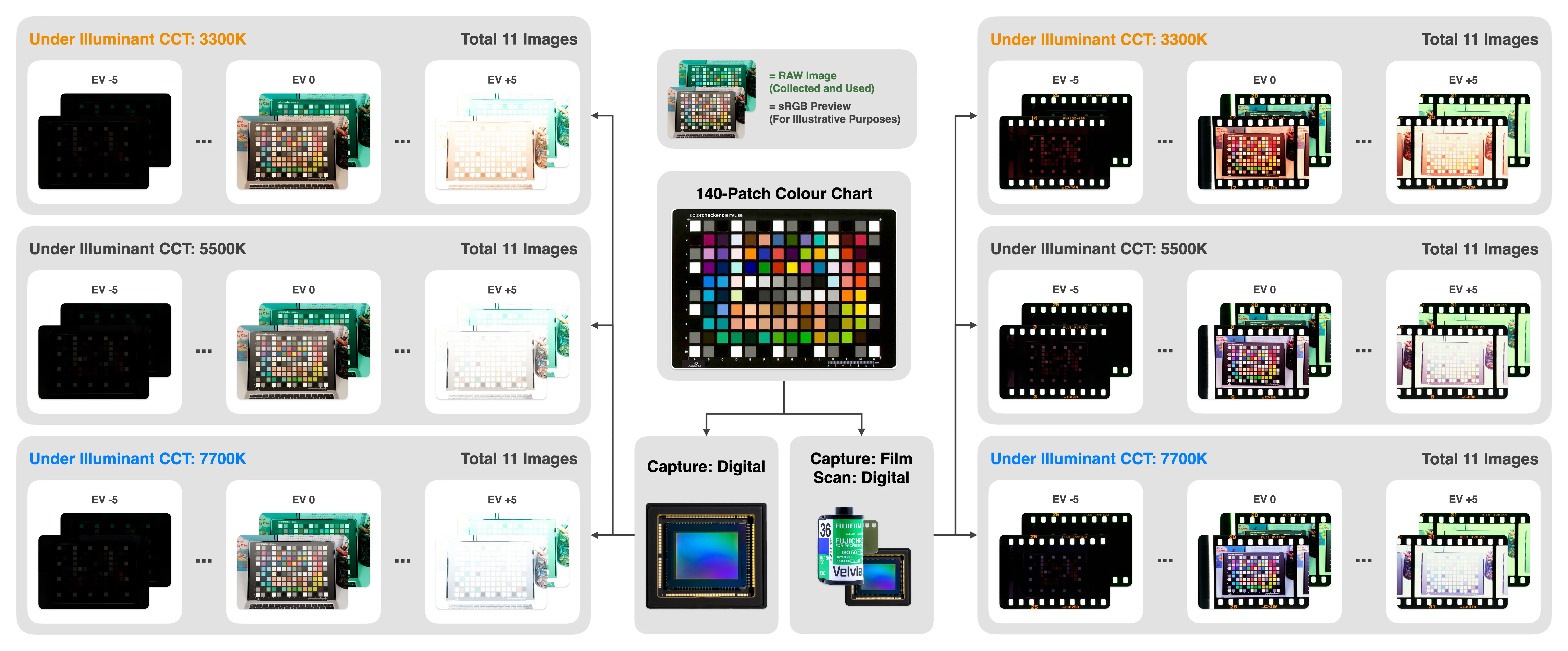
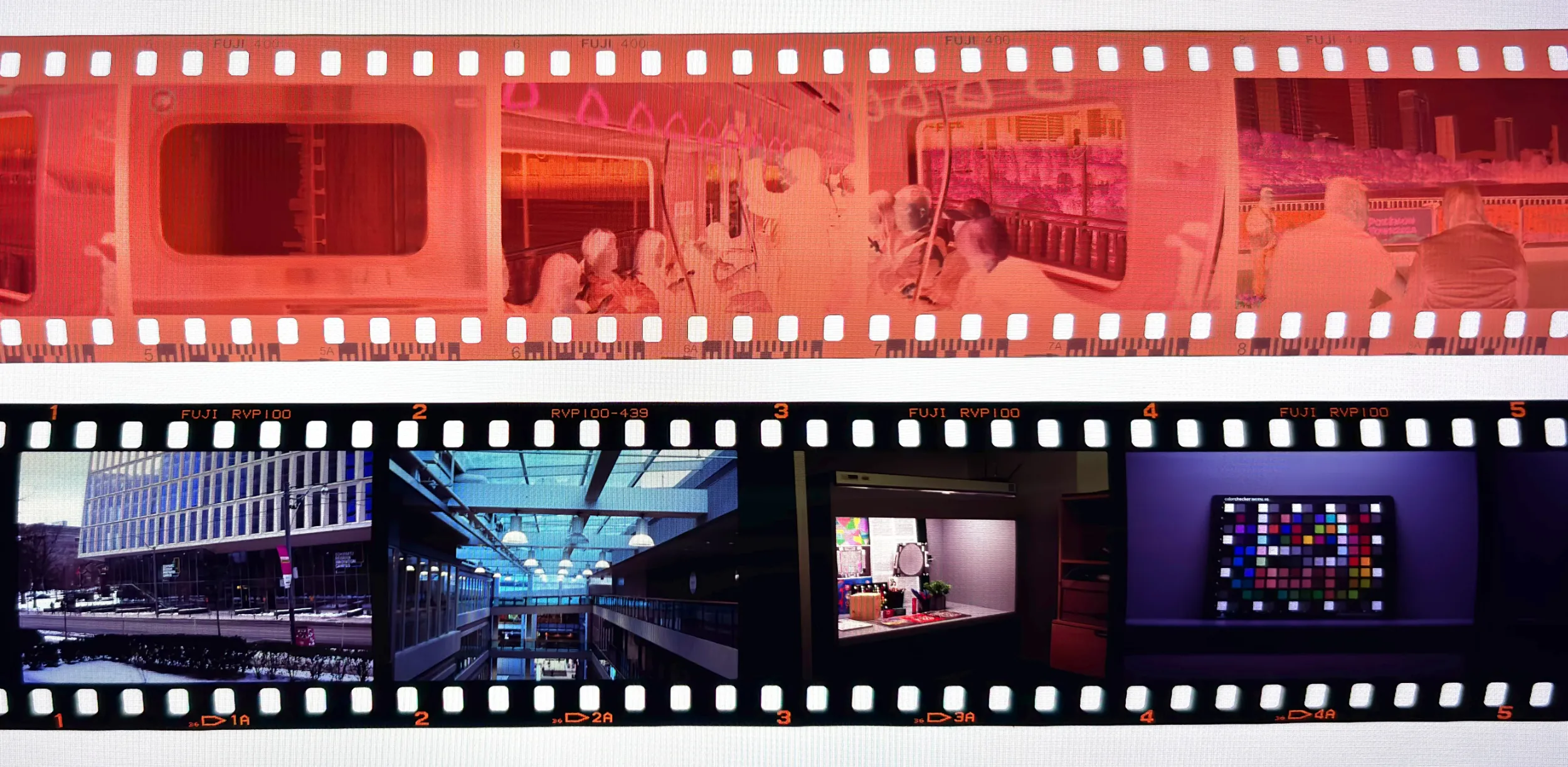
We trained and evaluated our model on Fujifilm VELVIA 100, a colour‑positive film renowned for its high saturation and characteristic reddish bias (Rockwell, 2007). VELVIA’s pronounced palette makes evaluation more reliable than subtler stocks. Both the digital scene‑capture and scanning devices were Fujifilm X‑PRO3 cameras. The film scene-capture device was NIKON F2AS. To generate many correspondences from a single 36‑exposure roll, we photographed the 140‑patch X-Rite Digital SG ColourChart under three distinct illuminants: correlated colour temperature (CCT) 3300K, 5500K and 7700K, and at 11 exposure levels in 1 exposure value (EV) steps. Exposure parameters (shutter speed, aperture, ISO) were synchronised between the two scene-capture cameras. The resulting data set comprises $3 \times 11 = 33$ image pairs and $33 \times 140 = 4620$ patch pairs. Excluding the replicated border patches leaves 3168 unique correspondences, sufficient to fit all 30 model parameters. For film scanning, we used a D50 backlight at $1000 \mathrm{cd/m^2}$. For each image we:

1. Computed a homography via four manual corner clicks to isolate the chart.
2. Averaged a square region inside every patch.

This workflow avoids pixel‑wise alignment and mitigates colour noise, motion blur and minor focus errors, keeping data capture simple enough for enthusiasts while yielding many correspondences.

Experimental results

Evaluation metrics and baselines

Our goal is an emulation such that, when a digital camera and a film camera capture the same scene under identical settings, the digital image processed through our model is perceptually similar to the scanned film. We therefore report both:

• Five‑fold cross‑validated root‑mean‑square error (RMSE) computed from emulated and ground truth values of the 140‑patch X-Rite Digital SG ColourChart.
• Qualitative visual inspection of real‑world scenes, because at the end of the day, this is what matters!

Baselines are:

1. End‑to‑end LUT (arbitrary function interpolator) a la (David, 2013), constructed directly from our captured data without any model fitting. This acts as an indicator to what results to expect without any priors.
2. Matrix + per‑channel tone curves inspired by digital radiometric calibration (Lin et al., 2011; Kim et al., 2012). Similar to our proposed model, but without the second matrix $M_{\mathrm{film} \rightarrow\mathrm{scan}}$. To confirm that conventional models for digital cameras cannot be re-used for film directly.

Quantitative results

Model	Five‑fold average RMSE across 140 patches
LUT (Baseline 1)	0.0111
Matrix + Curves (Baseline 2)	0.0149
Proposed Model ($M_{\mathrm{digital} \rightarrow \mathrm{film}}$ + Curves + $M_{\mathrm{film} \rightarrow\mathrm{digital}}$)	0.0116
Proposed Model (Alt.) ($M_{\mathrm{digital} \rightarrow \mathrm{film}}$ + Curves + $M_{\mathrm{digital} \rightarrow \mathrm{film}}^{-1}$)	0.0120

We notice that the LUT baseline, our propose model, and our alternative proposed model both perform similarly when tested on the 140-patch colour chart. The Matrix + Curves baseline performs slightly worse.

Qualitative results

However, RMSE alone does not paint the whole picture. Below are two example scenes, one outdoors and one indoors, rendered across the best-performing models from the quantitative results:

• LUT (Control) baseline reproduces colours but shows noticeable banding from sparse‑grid interpolation.
• Our proposed model closely match the ground‑truth digitised film with no visible artefacts.
• (Bonus) Fujifilm’s official “Film Emulation” feature on their digital cameras produces completely different colours.

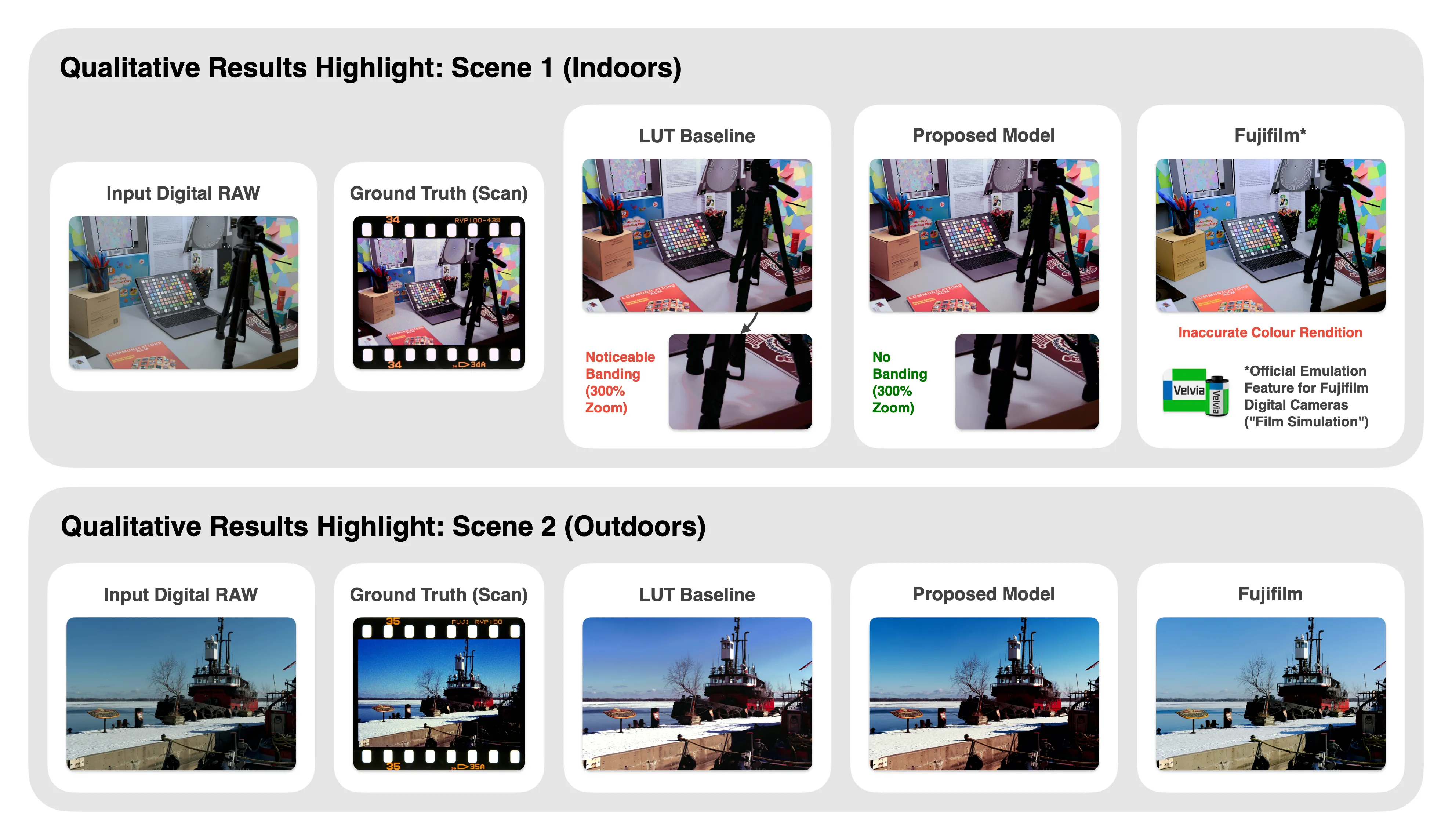
One might think: “If the only issue with a basic LUT constructed from captured point pairs is interpolation error, can’t you just capture more points and/or with better uniformity?”, to which we introduce one of our model’s unique advantages…

Interpretability of parameters

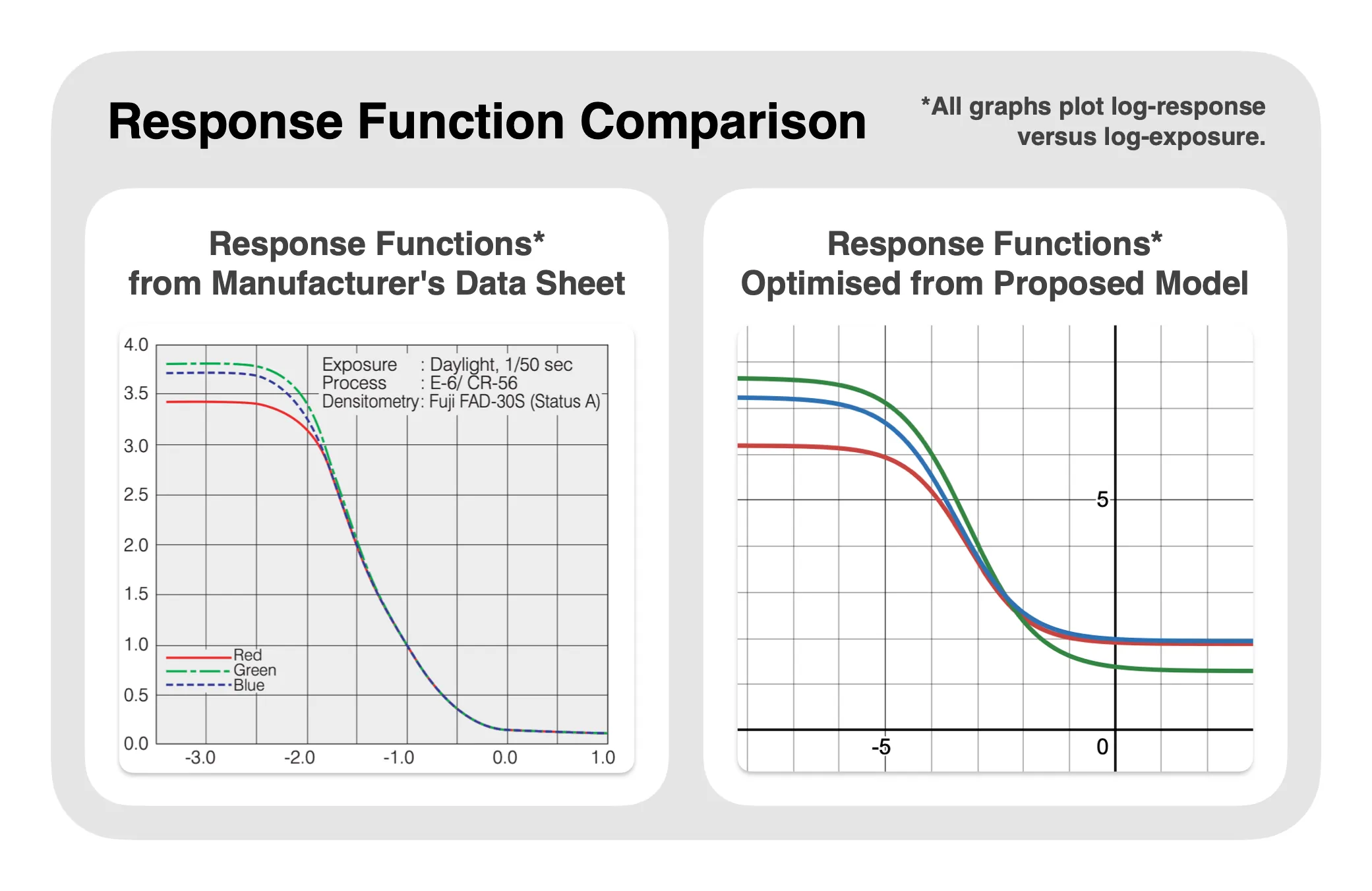
Notice that our model’s 12 curve (sigmoid) parameters ($A,k,x_0,y_0$ per channel) correspond directly to film characteristic curves. The above figure plots the optimised curves alongside the manufacturer data sheet for Fujifilm VELVIA 100. The ordering and shape of the red, green and blue curves align closely, validating the physical plausibility of the fitted parameters. Note that axis units may differ between physical density and RAW space. Unlike with black-box models, such interpretability may allow for some interesting use cases, such as physically-based tuning of the characteristic curves, or the derivation of curve parameters straight from the data sheet.

Discussion

Working in a Device‑Independent Space

The proposed model learns a mapping from digital‑camera RAW space $R_\mathrm{digital}$ to scanned-film RAW space $R_\mathrm{scan}$, both of which are sensor‑dependent. Consequently, inference requires the same sensor used during training. A simple remedy is to operate in a sensor‑independent colour space: e.g. CIE XYZ or ProPhoto RGB, before parameter optimisation. For every image pair in the data set we may apply the camera‑specific WB + CST (Fixed. No spatially dependent AWB, for example) matrices once to obtain sensor-independent values, then fit the model in that space. This is feasible because the matrices are fixed across the dataset and during inference, and film itself is deterministic as well as spatially independent. In practice, optimisation and evaluation in ProPhoto RGB produced metrics indistinguishable from RAW‑space, and the provided source code will also operate in ProPhoto RGB space.

Applications

• Aesthetic photofinishing: This is the main objective of the project. We wanted to build a film emulation technique that we could confirm that was accurate, by capturing real film and emulating each step in the real film capture-develop-scan process, without resorting to generic black-box models or using “fake” synthetic images. The benefits for emulation are already well known: film was engineered for decades to yield images that human observers find pleasing, and modern digital media can benefit from it. Our model offers such aesthetic as a deterministic, physically based transform requiring little user effort. Because the mapping is continuous, we can export discrete LUTs of any resolution and colour space, making the method a drop‑in replacement for workflows in cinematography or Adobe Lightroom.
• Film preservation: Many film stocks are being discontinued (National Geographic, 2010). However, we show that the capture of a single 36‑exposure roll plus our optimisation pipeline can digitally preserve the film’s colour signature. Combined with separate models for grain and halation, nearly the full look of a film can be archived for future generations!

Limitations

• No colour-negative film emulation: Our model targets colour‑positive film. Extending to scanned negatives (e.g. Kodak GOLD, Fujifilm SUPERIA) is feasible but requires an offset term for the orange base layer, and either an additional transform that mimics photographic printing or a direct model of the non‑inverted scanned negative RAW, leaving the final inversion task to downstream software.
• Need for more testing: Unfortunately, due to the scarcity of colour-positive film in the modern day as well as the cost of development, we were only able to utilise one 36-exposure roll of Fujifilm VELVIA 100 for this project. After the 33 colour chart captures and 1 buffer exposure, only two exposures remained for general scene evaluation.

Future Work: Derived Parameters?

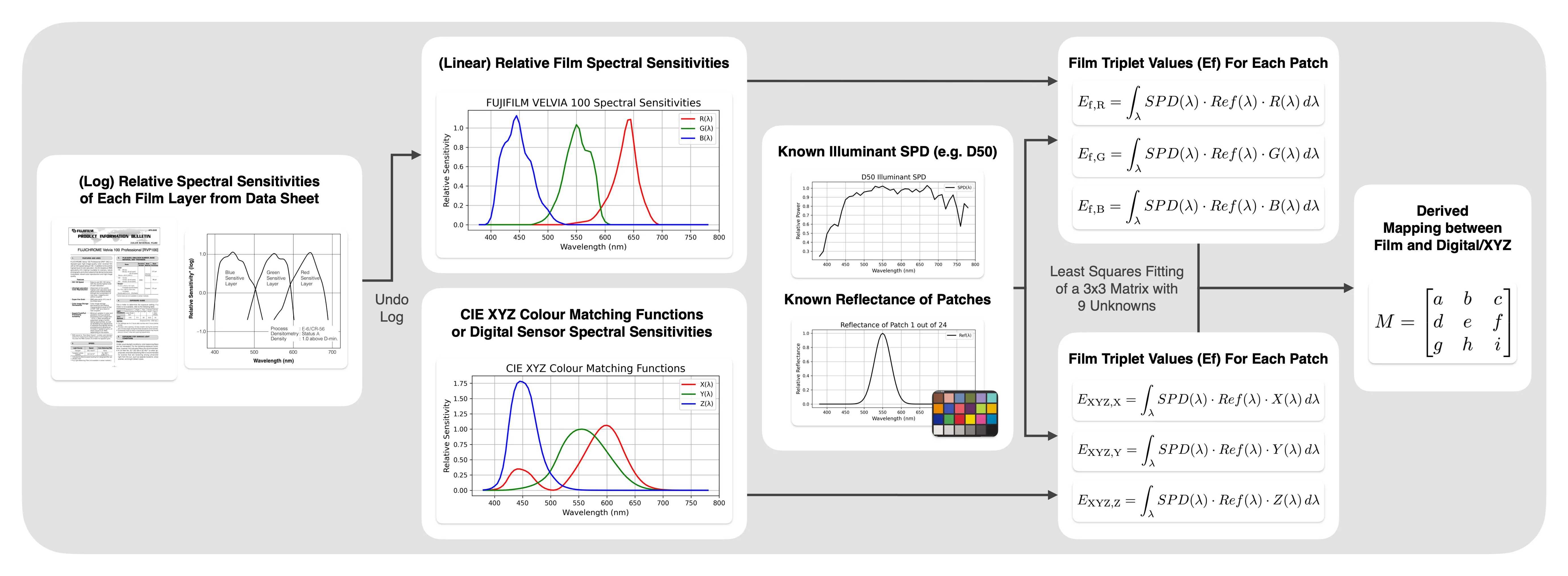
By design, both mapping matrices and the 12 characteristic curve parameters are grounded in some physical transformation. We also verify the latter through comparison with the manufacturer’s data sheet. Therefore, we hypothesise that all parameters may be completely derived from the data sheet alone, as the exact spectral sensitivities and characteristic curves are provided. This may allow the revival of long-lost discontinued film such as the famous Kodak KODACHROME without even capturing any data. While deriving the characteristic curve is straightforward (manual inspection, least squares, etc.), it cannot be said the same for the two matrices. Below is a hypothetical methodology for deriving either matrix based on the spectral sensitivities of film and a digital sensor (or colour-matching functions of XYZ), although yet to be experimented with.

Conclusion

We introduced a compact, physically grounded model for emulating colour‑positive film from digital images. By analysing the dual‑capture nature of scanned film and encoding it with two linear matrices and per‑channel sigmoids, we achieved accuracy on a par with and arbitrary interpolator LUTs while retaining interpretability and requiring only 1 film roll’s worth of captured image pairs for training. Experiments confirmed the necessity of the second matrix that models scanning and demonstrated visual fidelity on real‑world scenes.

References

• James Artaius. Here’s why fujifilm x100vi preorders are off the charts – and it’s a lesson for other camera companies. https://www.techradar.com/cameras/compact-cameras/heres-why-fujifilm-x100vi-preorders-are-off-the-charts-and-its-a-lesson-for-other-camera-companies, 2024. Accessed: 2025-04-16.

• Haiting Lin, Seon Joo Kim, Sabine Süsstrunk, and Michael S. Brown. Revisiting radiometric calibration for color computer vision. In 2011 International Conference on Computer Vision, pages 129–136, 2011.

• Seon Joo Kim, Hai Ting Lin, Zheng Lu, Sabine Süsstrunk, Stephen Lin, and Michael S. Brown. A new in-camera imaging model for color computer vision and its application. IEEE Transactions on Pattern Analysis and Machine Intelligence, 34(12):2289–2302, 2012.

• Arne M. Bakke, Jon Y. Harderberg, and Steffen Paul. Simulation of film media in motion picture production using a digital still camera. Image Quality and System Performance VI, vol. 7242, International Society for Optics and Photonics, SPIE, 2009.

• Zinuo Li, Xuhang Chen, Shuqiang Wang, and Chi-Man Pun. A large-scale film style dataset for learning multi-frequency driven film enhancement. In Proceedings of the Thirty-Second International Joint Conference on Artificial Intelligence (IJCAI-23), pages 1689–1696, International Joint Conferences on Artificial Intelligence Organization, 2023.

• Pierre Mackeenzie, Mika Sengehaas, and Raphael Achodou. Cnns for style transfer of digital to film photography, 2024.

• Pat David. Film emulation presets in g’mic/gimp. https://patdavid.net/2013/08/film-emulation-presets-in-gmic-gimp/, 2013. Accessed: 2025-04-16.

• LiftGammaGain forum user. Reverse-engineering fujifilm film simulations using a nn + lut. https://www.liftgammagain.com/forum/index.php?threads/reverse-engineering-fujifilm-film-simulations-using-a-nn-lut.18794/, 2024. Accessed: 2025-04-16.

• Dan Tseng, Yuxuan Zhang, Lars Jebe, Xuaner Zhang, Zhihao Xia, Yifei Fan, Felix Heide, and Jiawen Chen. Neural photo-finishing. ACM Trans. Graph., 41(6), 2022.

• Yuanming Hu, Hao He, Chenxi Xu, Baoyuan Wang, and Stephen Lin. Exposure: A white-box photo post-processing framework. ACM Trans. Graph., 37(2), 2018.

• Eastman Kodak Company. Basic photographic sensitometry workbook, 1999. Available from film data archives and enthusiast resources.

• Ken Rockwell. Fujifilm velvia 100. https://www.kenrockwell.com/fuji/velvia100.htm, 2007. Accessed: 2025-04-16.

• National Geographic. The end of kodachrome. https://www.nationalgeographic.org/the-end-of-kodachrome/, 2010. Accessed: 2025-04-16.